Ecoregions Maps in R

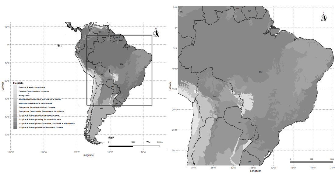
South American ecoregions with a zoom out to Brazil
by Russell J. Gray

Ecoregions maps are simple in R, here is some reproducible code to make them yourself. You can download the newest version (2017) WWF ecoregion data  here

code:
# make sure to set the working directory to  your folder that you have unzipped the  the ecoregions shapefile 
setwd("")

library(ggplot2)
library(rgdal)
library(ggspatial)
library(raster)
library(cowplot)
library(egg)
library(rnaturalearth)
library(sf)
library(hddtools)
#------------------------------------------------------------------------
# get a world object with all countries
world <- ne_countries(scale = "medium", returnclass = "sf")
world.SA <- subset(world, continent=="South America")
# get central points and coordinates to label the country names
# don't worry about the warning message it just refers to possible
# improper location of country name text (but insignificantly so)
world_points<- st_centroid(world)
world_points <- cbind(world, st_coordinates(st_centroid(world$geometry)))
SA <- subset(world_points, continent == "South America")
plot(SA)
Brazil <- subset(SA, iso_a3 == "BRA")
plot(Brazil)
#------------------------------------------------------------------------
list.files(pattern=".shp")
eco.regions <- readOGR(getwd(), "tm_ecoregions_2017")
# get ecoregions for Sout America
eco.regions.SA <- subset(eco.regions, REALM=="Neotropic")
eco.df <- fortify(eco.regions.SA, region ="BIOME_NAME")
#--------------------------------------------------------------
#---------------------------------------------------------------
# create a bounding box around Brazil
bbSP <- bboxSpatialPolygon(boundingbox = extent(Brazil))
# fortify the shape file
eco.simp <- crop(eco.regions, extent(bbSP))
eco.simp <- fortify(eco.simp, region ="BIOME_NAME")
table(eco.df$id)
#-----------------------------------------------------------------------------------
# Make the map
p1 <- ggplot() +
geom_spatial_polygon(data = eco.df, aes(x = long, y = lat, group = group, fill=id),
alpha = 1, linetype = 1) +
scale_fill_manual(values = grey.colors(13, rev = TRUE))+
geom_sf(data = world, fill= NA, lwd=1, color="black") +
geom_spatial_polygon(data = bbSP, aes(x = long, y = lat, group = group), size = 1.5,
alpha = 1, linetype = 1, color = "black", fill = NA) +
geom_sf(data = world.SA, fill= NA, size = 0.5) +
geom_text(data= SA,aes(x=X, y=Y, label=wb_a3), size = 2,
color = "black", fontface = "bold", check_overlap = FALSE) +
annotation_north_arrow(location = "tr",
which_north = "true",
pad_x = unit(0.3, "in"),
pad_y = unit(0.35, "in"),
style = north_arrow_fancy_orienteering) +
ggsn::scalebar(x.min=-30, x.max=-50, y.min=-57, y.max=55, transform = TRUE,
dist = 1000, dist_unit = "km", location = "bottomright",
box.fill = c("black", "white"), st.color = "black",
height = 0.005, st.bottom = FALSE, st.size = 2.5) +
coord_sf(xlim = c(-120, -26.24139), ylim = c(-58.49861, 12.59028),
expand = FALSE) + xlab("Longitude") + ylab("Latitude") +
ggtitle("") +
theme(panel.grid.major = element_line(color = gray(.5),
linetype = "dashed", size = 0.5),
panel.background = element_rect(fill = "white"),
legend.title = element_text(face=2),
legend.background = element_blank(),
legend.key = element_blank(),
legend.position = c(.01, .15),
legend.justification = c("left", "bottom"),
legend.box.just = "left",
legend.text = element_text(size=8,face=2))+
labs(color="Species",fill = "Habitats")
p1
p2 <- ggplot() +
geom_spatial_polygon(data = eco.simp, aes(x = long, y = lat, group = group, fill=id),
alpha = 1, linetype = 1) +
scale_fill_manual(values = grey.colors(13, rev = TRUE))+
geom_sf(data = world, fill= NA, lwd=1, color="black") +
geom_sf(data = world.SA, fill= NA, size = 0.5) +
geom_text(data= SA,aes(x=X, y=Y, label=wb_a3), size = 2,
color = "black", fontface = "bold", check_overlap = FALSE) +
annotation_north_arrow(location = "tr",
which_north = "true",
pad_x = unit(0.3, "in"),
pad_y = unit(0.35, "in"),
style = north_arrow_fancy_orienteering) +
ggsn::scalebar(x.min=-35, x.max=-50, y.min=-33, y.max=1, transform = TRUE,
dist = 500, dist_unit = "km", location = "bottomright",
box.fill = c("black", "white"), st.color = "black",
height = 0.005, st.bottom = FALSE, st.size = 2.5) +
coord_sf(xlim = c(-74.00205, -34.80547), ylim=c(-33.74219, 5.257959),
expand = FALSE) + xlab("Longitude") + ylab("Latitude") +
ggtitle("") +
theme(panel.grid.major = element_line(color = gray(.5),
linetype = "dashed", size = 0.5),
panel.background = element_rect(fill = "white"),
legend.title = element_text(face=2),
legend.background = element_blank(),
legend.key = element_blank(),
legend.position = "none",
legend.justification = c("left", "bottom"),
legend.box.just = "left",
legend.text = element_text(size=8,face=2))+
labs(color="Species",fill = "Habitats")
p2
plot_grid(p1,p2,ncol = 2,nrow = 1)