|
Author: Russell Gray 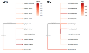 ***Check out R Bloggers (https://www.r-bloggers.com) for more tutorials and walkthroughs on your analyses*** Required Data obtained from: http://snakedatabase.org/pages/ld50.php
Required packages remotes::install_github("GuangchuangYu/treeio") install.packages("BiocManager") BiocManager::install("ggtree") You will need to use the Install.Packages() function before you open these in the library library("ape") library("taxize") library("rentrez") library("phytools") library("select") library("treeio") library("ggtree") library("data.tree") library("tidytree") library("ggplot2") library("dplyr") This book is super helpful I encourage everyone to check it out! https://yulab-smu.github.io/treedata-book/chapter2.html ############################################################# #Set your workdesk setwd("C:/Users/Russell/Desktop/venom") This is the attached data file from above #read in your data with species names and traits you would like to use dat<-read.csv("TBLld50.csv") #pull the species names column out to create a species list string sp_list<-as.character(dat$Scientific.Name) #set your ncbi key. If you don't have one, you can get it #by registering an account with ncbi set_entrez_key("xxxxxxxxxxxxxxxxxxxxxxxxxxxxxxxxxxx") Sys.getenv("ENTREZ_KEY") #obtain cladistic data on your species list from ncbi taxise_sp <- classification(sp_list, db = "ncbi") #Coerce your species list into a classtree object tax_tree <- class2tree(taxise_sp) #Pull the phylo object from the classtree for plotting tax_phylo <- tax_tree$phylo #plot your basic tree to see what it looks like change x/y values according #to your own data new.snake.tree %>% ggtree() + geom_tiplab(size=1) + theme_tree2() + xlim(0, 90) 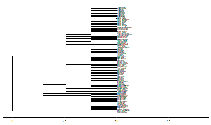 #Now that the tree works lets write it into a newick file in case #we need it later write.tree(tax_phylo, file = "Snake_Tree") #import the tree file again just to make sure the function works #give it an appropriate name for your species (note: this function works with several different tree files, so if you have the ability to import a n existing tree with proper branch distance metrics, that would be ideal) snake.tree <- read.newick(file = "Snake_Tree") #now lets try to subset the tree in case we want to check some #target species #check names of tips to use in sample subset head(snake.tree$tip.label) #make a subset of the tree and highlight a species #levels back represents cladistic level (family, superfamily, order, class etc.) snake.treeub<-tree_subset(snake.tree, "Hydrophis_viperinus", levels_back = 2) snake.treeub %>% ggtree(aes(color = group)) + geom_tiplab(size=2) + theme_tree2() + scale_color_manual(values = c(`1` = "red", `0` = "black")) + xlim(0, 80) 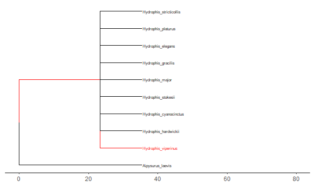 #break the tree into its basal parts as a tibble tibtree <- as_tibble(snake.tree) #remove that "_" from between the genera and specific epithet tibtree$label <- sub("_", " ", tibtree$label) #keep only the species, total body length, and ld50 data #we want in the "dat" data frame, have to divide for different trees #or else the combination will produce NA and errors (i don't know why) dat <- select(dat, Scientific.Name, IV..mgkg., TBL..cm.) #change column names for joining colnames(dat)[colnames(dat)=="Scientific.Name"] <- "label" colnames(dat)[colnames(dat)=="IV..mgkg."] <- "LD50" colnames(dat)[colnames(dat)=="TBL..cm."] <- "TBL" dat$label<-as.character(dat$label) #convert to tibbles for each type of trait tibdat<-tibble(label=paste0(dat$label), LD50=dat$LD50, TBL=dat$TBL) library(stringr) #remove any invisible characters (for some reason this happens) tibdat$label<-str_replace_all(tibdat$label, "[^[:alnum:]]", " ") tibtree$label<-str_replace_all(tibtree$label, "[^[:alnum:]]", " ") #remove leading/trailing spaces from the data #returns string w/o leading or trailing whitespace trim <- function (x) gsub("^\\s+|\\s+$", "", x) tibdat$label<-trim(tibdat$label) tibtree$label<-trim(tibtree$label) #add traits to the tree tibble we just made and merge using #scientific name column "label" tib_tree <- full_join(tibtree, tibdat, by.x = "label") #reclassify the tibble columns again (annoying but necessary) tib_tree$parent<-as.integer(tib_tree$parent) tib_tree$node<-as.integer(tib_tree$node) tib_tree <- tib_tree[c("parent","node","branch.length","label","LD50", "TBL")] #make sure everything is good for conversion tib_tree class(tib_tree) #remove duplicates (in case there are any) tib_treeND<-unique(tib_tree) #convert into phylo object with trait data as a feature new.snake.tree<-as.treedata(tib_treeND) #check names to use for subset new.snake.tree@phylo$tip.label #subset the tree data (ignore the warning) #if you try to plot the whole tree it won't work, I'm still unsure why that is treesub_new<-tree_subset(new.snake.tree, "Crotalus scutulatus", levels_back = 3) #plot the tree with LD50 values as colors on the branches ggtree(treesub_new, aes(color=LD50), ladderize = TRUE,right = FALSE, continuous = FALSE, size=1) + scale_color_distiller(palette = "Reds", direction = 1) + geom_tiplab(hjust = -.1, size=1.8, color = "black") + geom_nodelab(aes(x=branch), size=2.5, vjust=-0.5)+ geom_tippoint() + theme(legend.position = c(0.80, .85))+ xlim(0,70) 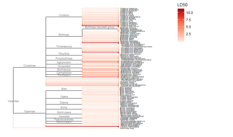 #plot a tree with Total Body Length (TBL) on the branches ggtree(treesub_new, aes(color=TBL), ladderize = TRUE,right = FALSE, continuous = FALSE, size=1) + scale_color_distiller(palette = "Reds", direction = 1) + geom_tiplab(hjust = -.1, size=1.8, color = "black") + geom_nodelab(aes(x=branch), size=2.5, vjust=-0.5)+ geom_tippoint() + theme(legend.position = c(0.80, .85))+ xlim(0,70) 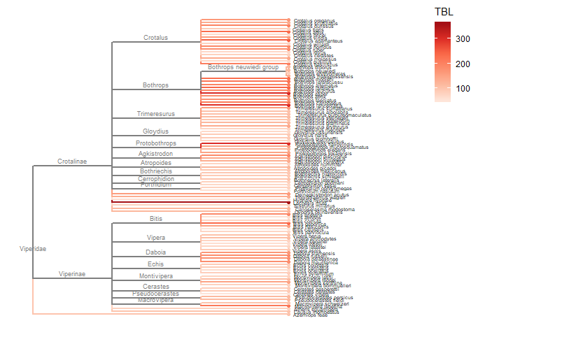 #resub and do a sidebyside to see if you can visualize any correlations #also lets change the species to some Hydrophis for a smaller subset treesub_new<-tree_subset(new.snake.tree, "Hydrophis viperinus", levels_back = 2) #plot the tree with LD50 values as colors on the branches p1<-ggtree(treesub_new, aes(color=LD50), ladderize = TRUE,right = FALSE, continuous = FALSE, size=1) + scale_color_distiller(palette = "Reds", direction = 1) + geom_tiplab(hjust = -.1, size=2.5, color = "black") + geom_nodelab(aes(x=branch), size=2.5, vjust=-0.5)+ geom_tippoint() + theme(legend.position = c(0.90, .85))+ xlim(0,70) #plot a tree with Total Body Length (TBL) on the branches p2<-ggtree(treesub_new, aes(color=TBL), ladderize = TRUE,right = FALSE, continuous = FALSE, size=1) + scale_color_distiller(palette = "Reds", direction = 1) + geom_tiplab(hjust = -.1, size=2.5, color = "black") + geom_nodelab(aes(x=branch), size=2.5, vjust=-0.5)+ geom_tippoint() + theme(legend.position = c(0.90, .85))+ xlim(0,70) library(cowplot) #side by side to check any correlation plot_grid(p1, p2, ncol = 2, nrow = 1, labels = c("LD50", "TBL")) 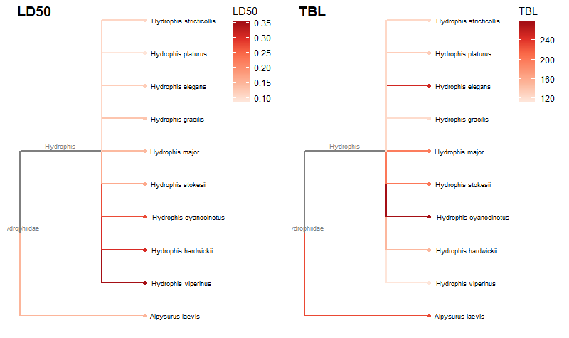 R Code for this tutorial
AuthorRussell J. Gray
1 Comment
|
AuthorRussell J. Gray Archives
April 2021
Categories |
||||
 RSS Feed